Geographic Information System (GIS) methodologies are an essential tool for glacial research looking to understand the spatial distribution and character of landforms. While manual mapping can typically be done, to optimize the use of large his resolution data sets a more efficient approach is necessary. To examine large swathes of glacially influenced terrains across North America, the Planet Earth Lab developed an approach to automate the mapping of glacial landforms termed Curvature-Based Relief Separation (or CBRS for short). This allowed for the transformation of raw digital elevation model (DEM) to polygons representative of possible glacial landforms such as drumlins or MSGLs (Mega Scale Glacial Lineation). This has led to many new projects and publications striving to understand the evolution of glacial landforms.
Sounds familiar but forget what a drumlin is? A quick refresher on drumlins can be found in the post here
Check out the recent publication from the Planet Earth Lab showing the results of automated surface mapping here
How do we go from raw data to mapped terrains?
The CBRS approach can be broken down into seven distinct steps evolving raw DEM data to mapped polygons that can be evaluated with further analytical tools to extract relevant characteristics.
The first step is to acquire digital elevation model (DEM) data for your study area (Figure 1). Already at this step the landforms are visible and can undergo manual mapping, albeit taking more time. Prior to automated CBRS mapping the raw data undergoes smoothing using focal statistics to make a more cohesive and continuous surface for the subsequent analysis (Figure 2).
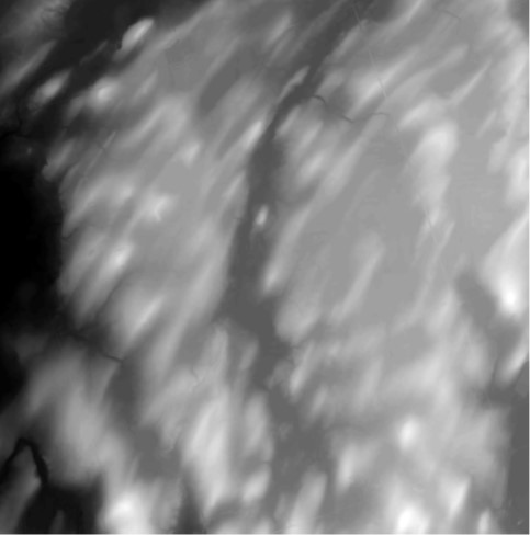
Figure 1- Raw DEM data
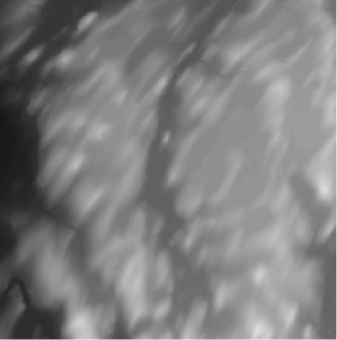
Figure 2- Smoothed DEM data after applying focal statistics
The smoothing of the DEM surface is an essential operation that aids the next step where the calculation of the surface’s curvature is carried out (Figure 3). Since curvature is a function of slope, the smoothing of the surface in the previous step reduces the incidence of discontinuities which are problematic for slope calculations. Following calculation of the surface’s curvature the breaks in the curvature are traced (Figure 4). Visually the outline of the glacial landforms are already starting to take shape. To convert these outlines to useable polygons the curvature breaks are interpolated and then subtracted from the DEM (Figure 5) producing a raster that then undergoes fuzzy classification and conversion to polygons (Figure 6).
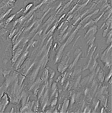
Figure 3- Output following the calculation of the surface's curvature
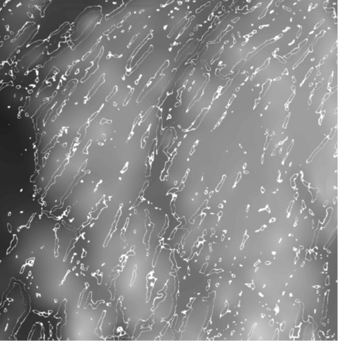
Figure 4- Lines delineating the break in slope on the curvature surface
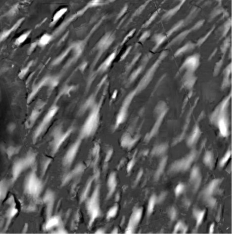
Figure 5- Interpolating break of slope and subtracting from DEM
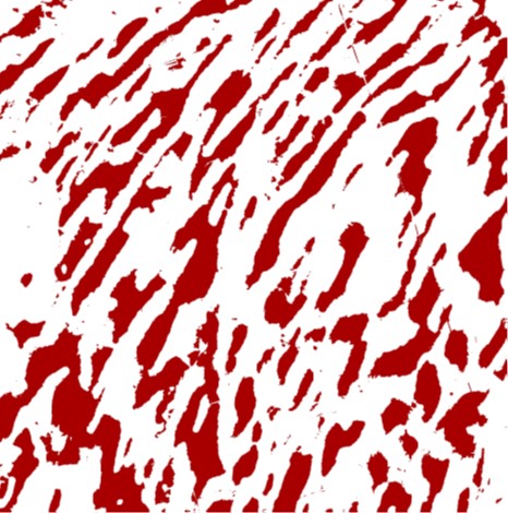
Figure 6- Features defined following fuzzy classification and raster conversion
Quality control is conducted manually after polygons are automatically generated. This helps eliminate spurious or erroneous polygons. Afterwards, functions can be applied to the polygons to rapidly tabulate elongation ratios, for example, which are crucial indicators for understanding the genesis of the glacial landforms (Figure 7).
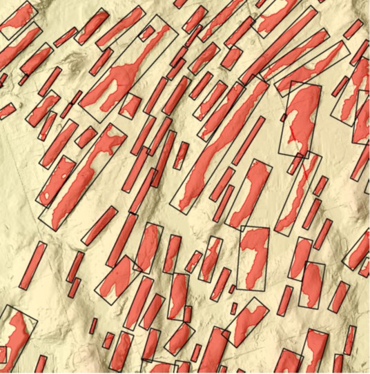
Figure 7- Output following removal of spurious polygons allowing for further analysis such as the calculation of the elongation ratios for each feature
So what does this mean?
The means to objectively identify glacial features automatically allows for the mapping of glacial morphotypes over large areas. This has been shown to have a marked impact of the number of features identified. This is particularly the case for features with high elongation ratios, think long and thin, such as MSGLs. For example, in the areas surrounding the Oak Ridges Moraine, using previous mapping techniques only 1% of landforms were classified as MSGLs while the CBRS methodology revealed they were a lot more common at 20% of landforms. CBRS has therefore shown that it can be a valuable tool to help supplement the weary eyes of researchers investigating past glacial landscapes!